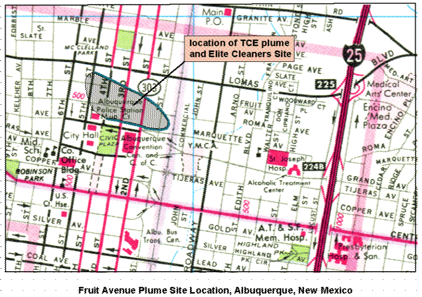
The site chosen by the Bernalillo County Environmental Health Department
for the Smart Sampling component of the 1997 TDI is known as the Fruit
Avenue Plume, located in downtown Albuquerque, New Mexico. At present,
the New Mexico Environment Department (NMED), under direction of the United
States Environmental Protection Agency (EPA), is continuing its investigation
of the chlorinated solvent groundwater plume at this site (CERCLIS #NMD986668911).
The NMED has received funding from the EPA to determine the extent and
source(s) of the plume and the NMED's 1997 work plan includes the installation
of additional monitoring wells. The work plan, which specifies the
locations of additional monitoring wells to be drilled, was already established
and approved prior to the TDI. Therefore, the results from this analysis
(the identification of optimal locations for placing additional monitoring
wells) may be used to augment or modify the existing sampling design depending
on the progress of the current drilling program. It should be noted
that this work was performed independently of the on-going drilling program
and that the author had no knowledge of the additional sampling locations
chosen by NMED staff prior to the submission of this report.
BACKGROUND
In 1989, TCE and PCE contamination exceeding Maximum Contaminant Levels
(MCLs) was discovered in the Coca-Cola Bottling Company's production well;
the well was subsequently shut down. Investigations conducted by
NMED in 1989, 1990 and 1993 confirmed the presence of a chlorinated solvent
plume in the aquifer. The plume is known to exist between Broadway
and 5th streets and between Lomas Boulevard NW and Marquette Avenue.
The initial investigations focused on the Elite
Cleaners site, formerly located between Second and Third Street, and
Roma and Lomas Boulevard. Two underground storage tanks believed
to have contained solvents used for the dry cleaning activities conducted
between the 1940s and 1972, were removed in 1989.
Groundwater investigations conducted in 1993 by the NMED and Norwest
Corporation, which was interested in purchasing property in the area, showed
that the contamination was more widespread than previously thought.
The monitoring wells are completed
at three depths: 14 wells are screened in the shallow zone (about 40 feet
bgs), eight wells in the intermediate zone (about 85 feet bgs), and two
in the deep zone (greater than 110 feet bgs). In 1993, the highest
concentrations were found in well DM-12(I), more than 1000 feet upgradient
of the Elite Cleaners site, hence additional sources of the TCE are suspected.
TCE conconcentrations exceeded the MCL of 5 ppb in eleven other wells sampled
in 1993. In December 1996, 23 wells were sampled for volatile organic
compounds (VOCs); of these, 17 wells contained detectable quantities of
TCE with six of these exceeding the MCL. At present, the highest
concentration of TCE is found in well DM-13(I) which is located on the
former Elite Cleaners property. The NMED investigations have concluded
that the water levels, hydraulic gradients and flow directions appear unchanged
from the 1993 conditions, and that the plume appears to be stabalized,
i.e., it does not show signs of significant vertical or lateral movement
since the 1993 sampling event.
LIMITATIONS
The level of funding allocated for this work was limited to the degree
that it was not feasible to perform the full Smart
Sampling methodology. The analyses performed involved components
of the Smart Sampling methodology that would be used in the first phase
of such an investigation. The result of this initial phase of the analysis
is the identification of optimal locations for the placement of additional
monitoring wells.
Because there is no cost information on the remediation of the plume (presumably a pump and treat scenario), it is not possible to use the Smart Sampling methodology to quantify the number of additional measurements to obtain in order to minimize the total expected cost of remediation (which includes the cost of the obtaining additional samples). Hence, the analyses have been conducted with the goal of better characterizing the extent of the plume which resides above the MCL which is 5 ppb for TCE. The optimal locations would be different if, for example, the goal was to characterize the plume where the plume "boundary" is defined by the detection limit (1 ppb).
The scope of work was limited to the analysis of TCE concentrations within the intermediate-depth zone where the concentrations are highest, and where, unfortunately, the data are more sparse (only eight measurements). Also, it is clear, from the data that have been collected thus far, that additional, unidentified sources are very likely to exist. It is therefore also likely that the process (the TCE contamination) is "nonstationary" meaning that its statistics, such as its mean and covariance properties, may vary as a function of location. While the assumption of stationarity is a basic premise of the geostatistical techniques employed in the analyses, the data are too few to assess whether this assumption is violated.
Performing geostatistical analyses on a data set of such a limited extent
will, no doubt, "raise eyebrows" among those in the geostatistical community
intimately familiar with the assumptions, limitations, and applicability
of geostatistical methods in the earth sciences. Clearly, a liberal
amount of "artistic license" was necessary to exercise this methodology
on this limited data set, but the intent was to introduce these concepts
to practicing environmental scientistists and bridge the gap between state-of-the-art
and state-of-practice. Given the current funding and data constraints,
the goal of this exercise is to demonstrate the potential usefulness of
this technology so that it might be utilized to advantage when a more appropriate
quantity of initial data are available or that it may be considered for
deployment at other sites.
DATA ANALYSIS AND SIMULATION
The data provided for this investigation by the NMED included an April,
1997 Groundwater Sampling Summary Report (NMED, [1997]), an historical
measured concentrations data table entitled "Summary of Groundwater Analytical
Results (ppb) - Fruit Avenue Plume Site" and a table of well completion
and water level data, a table of state plane coordinates for the majority
of the wells, and a sketch of vertical groundwater movement and TCE concentrations
in the Coca Cola well. The summary report includes contour
maps of water levels and TCE concentrations for two aquifer zones,
the shallow zone and the intermediate depth zone.
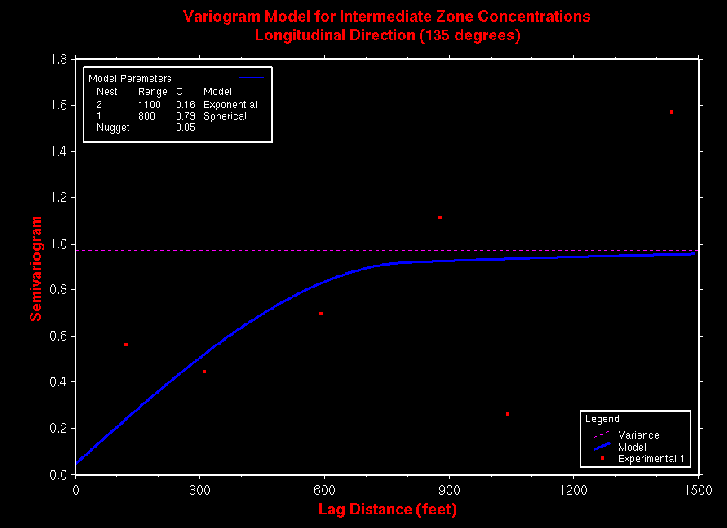
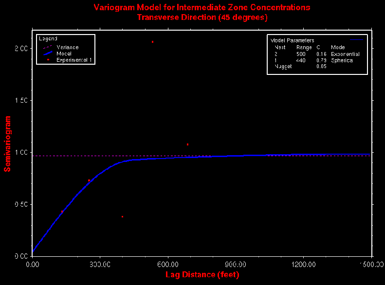
Semivariogram Analysis and Model Fitting
The analysis begins with empirical semivariogram estimates of the measured
TCE concentrations. The semivariogram characterizes the spatial variability
of the field variable (in this case, the TCE concentration); it quantifies
how different the measured values are likely to be as the separation distance
between the sampling points increases. The semivariogram is essentially
a "variance of differences" in the values as a function of the separation
distance. This variance therefore increases as the separation distance
increases. Semivariogram modeling attempts to capture the manner
in which this variability changes with separation distance, the magnitude
of the variability and the range or distance at which two points become
completely uncorrelated.
The hand-contoured TCE concentrations exhibit an anisotropic nature, where the values are correlated over a longer distance in the direction of groundwater flow. This is consistent with the type of spreading of the plume that one might expect to observe as a result of longitudinal and transverse dispersion. Consequently, while the data are sparse, directional variography was performed and a semivariogram model was fit to the two empirical semivariograms, one in the longitudinal direction oriented at 135 degrees clockwise from north, and the other in the transvere direction, oriented at 45 degrees. While there is significant scatter in the empirical semivariograms (the points on the graphs), these few data do, somewhat surprisingly, reflect the anisotropic character of the concentration data.
It should be noted that the TCE concentration data underwent a Gaussian
transformation (i.e., the data were transformed to a zero mean, unit variance
distribution) prior to the semivariogram analysis, consequently, the variance
approaches the value of 1.0 on the semivariogram plots. The reason
for this is that the simulation routine, SGSIM (Sequential Gaussian SIMulation),
is based on a multivariate normal distribution assumption. The semivariogram
analyses and model fitting was performed with the UNCERT code (Wingle,
et al., [1994]).
Monte Carlo Simulation of the TCE Concentration Distribution
The anisotropic model of the spatial variability (the blue line in
the semivariogram plots) exhibited by the TCE measurements was used in
the SGSIM code (Deutsch and Journel, [1992]) to generate realizations
of contaminant concentration fields that 1) have a Gaussian distribution,
2) honor the measured data at their respective locations, and 3)
exhibit the same spatial statistical behavior, i.e., have the same mean
and covariance properties, on average. One hundred such realizations
of the TCE concentration plume were generated in a sequential fashion,
a process which is referred to as Monte Carlo simulation. The fields
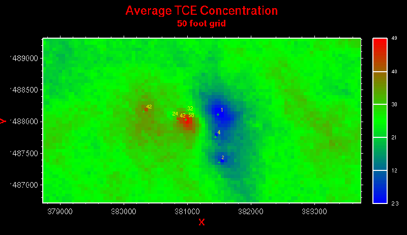
were generated on a regular grid or mesh having 20 foot spacings; initially,
a 50 foot grid was used but the plume boundary is better resolved with
the finer grid.
The plume was simulated over the entire area illustrated in the hand-contoured maps. The data, however, are clustered primarily in the central region of that area, consequently, there is no conditioning information (measurements) in the corners of the map (in the southwest, the northwest and eastern portions of the site). The average concentration is computed by averaging the simulated values at each point over the ensemble of realizations. The average concentration on the 50 foot grid shows values generally in the 20-30 ppb range, whenever the distance from the point being simulated and the conditioning data exceeds the correlation range of the data (about 1000 feet in the longitudinal direction). This occurs at the periphery but over a large portion of the field. What is occurring is the algorithm has no conditioning information in these far-removed-from-data locations, hence it draws a value randomly from the raw histogram of the data. The eight data values are 1, 2, 2, 4, 24, 32, 42, and 58, the average of which is 20, although the histogram may be skewed slightly to the high side (there are too few data to compute and plot the histogram). The simulated fields are thus unrealistic in these fringe areas, as is the average concentration field.
One way of dealing with this problem would be to add "fake conditioning data" in the fringe areas; these would be zero concentration values placed in locations where it is "known" (via expert judgement) that the plume does not exist. The problem is, in an area such as downtown Albuquerque, it is risky to assume no contamination exists at certain points, even if they are very far removed from the plume under investigation because of the possibility of encountering a plume from a different source. This is evident from the high concentration value found in well DM-12(I), 1000 feet upgradient of the Elite Cleaners site.
For expedience, the simulation algorithm was modified to simply ignore
the far-removed locations during the simulations, i.e., the value is not
simulated if the conditioning data are too far away. The result of
such an approach is shown by the average
concentration field on the 20 foot grid where the TCE plume is
only mapped in the vicinity of the conditioning data. Again, what
is probably not realistic about this representation is that the
edges of the plume should be showing decreasing values for the TCE concentrations.
This reinforces the fact that geostatistics is a tool for interpolation
of data, not extrapolation.
ANALYSIS OF THE SIMULATED FIELDS
Now that an ensemble of TCE concentration maps have been simulated,
the next step is to analyse these fields and characterize the nature of
TCE plume in a probabilistic manner. The results from this part of
the analysis are used to optimally select additional monitoring well locations.
Probability Mapping and Analysis
In this stage of the analysis, the simulations of the TCE concentration
field are analysed to identify areas of greatest uncertainty; then further
analyses are conducted to identify specific locations within those uncertain
areas where additional sampling wells should be optimally placed.
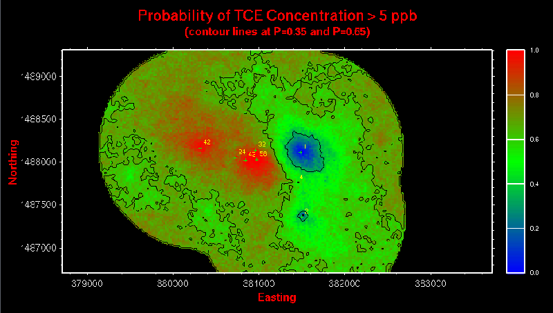
A probability map is derived from the ensemble of simulations by
computing the probability of exceeding a specified threshold at each location
in the simulated field (in this case the threshold is the MCL for TCE =
5 ppb). For example, if, at a particular location, 15 out 100 realizations
had TCE values in excess of 5 ppb, the probability value for this location
would be 0.15.
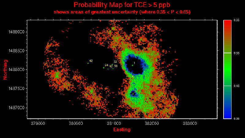
The probability map derived from these simulations shows the likelihood (probability) of the TCE concentration exceeding 5 ppb. The areas in which the probability is either very high or very low are not of much interest because these are fairly certain areas, where the level of contamination relative to the 5 ppb threshold is "known" with some degree of confidence. The areas of highest uncertainty would be those following the 0.50 probability contour line, where it's a "50-50 chance" that the contamination will exceed the MCL. Thus, the probability map was processed to show only the areas of greatest uncertainty defined by all points whose probability of exceedance lies between 0.35 and 0.65.
Identifying Optimal Sampling Locations
Within the area defined by the 0.35 and 0.65 probability of exceedance
values, there are many choices for placing additional monitoring points.
Consider for a moment all the grid cells crossed by the 0.50 probability
contour line; each of these cells had 50 realizations in which the simulated
TCE concentration was greater than 5 ppb and 50 realizations where the
concentration was less than 5 ppb. But the distribution of
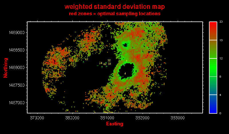
simulated concentrations at each of these points will vary; in particular,
the variance of some cells will be greater than the variance at other locations
along the 0.50 probability contour. It is the locations with the
higher variance that are the more uncertain, and would therefore have a
greater chance of reducing the total uncertainty if an additional monitoring
well were placed there.
Thus, a standard deviation map (derived
by taking the square root of the variance at each simulation grid cell)
is used in combination with the probability map information by an algorithm
called the "Weighted Standard Deviation Method" (McKenna, [1997])
to generate the final map of optimal additional sample locations.
In the WSDM approach, the standard deviation of TCE concentrations at a
given location is scaled by the factor F = 1 - 2 * | prob[i,j] - 0.5 |.
When the exceedance probability at grid cell location i,j is 0.5 (uncertainty
is largest), F=1.0 and as prob[i,j] approaches either 0 or 1, the scale
factor F approaches zero. The resulting weighted
standard deviation map indicates which areas within the .35 to .65
probability of exceedance zones are more optimal for locating additional
monitoring wells.
The final step is to take into account constraints on the placement
of wells, which, in the case of the Fruit Avenue Plume site, are significant.
Because the site is located in downtown Albuquerque, New Mexico, locations
suitable for drilling are limited because streets and buildings are excluded.
This leaves essentially sidewalks and parking lots. After the suitable
areas for drilling are identified and overlaid on the weighted standard
deviation map, specific locations for placing additional monitoring wells
can be selected. The well locations are selected from those areas
having the higher weighted standard deviation values with the additional
constraint that wells should not be placed too close to each other, in
order to avoid obtaining redundant information.
RESULTS
The existing work plan includes the drilling of 20 additional monitoring
wells clustered at various locations where each well in the cluster will
be screened at a different depth. About half of these will be screened
in the intermediate zone. Therefore, 10 additional sampling locations
were selected as recommended sites for additional sampling points based
on the results from these analyses. The suggested additional sampling
locations are shown on a map with the streets and
buildings overlain.
The sites were chosen by targeting those areas with the higher weighed standard deviation scores while trying to keep the wells separated as much as possible. The suggested sampling points generally circumvent the Elite Cleaners site and are located generally along the edge of streets. The one well on Marquette about two blocks west of Broadway probably should have been placed further to the south (on Grande) and closer to Broadway as it may provide some redundant information with that obtained from well DM-7(I). The other wells are placed in areas where the "edge of the plume" is not well defined based on the existing data of eight measurements.
It is not clear why the area between the labels for the Doubletree Hotel and Tijeras Avenue is "white" (does not rank as an important area of uncertainty which is likely to exceed the MCL). Given that there is no nearby conditioning data, it may be simply an artifact of results based on the analysis of a data set which is insufficient to provide reliable detailed simulations. There is a similar area north of Lomas Boulevard between 2nd and 3rd streets.
SUMMARY AND RECOMMENDATIONS
The Smart Sampling methodology was selected by the Bernalillo County
Environmental Health Department as a promising DOE-sponsored technology
for aiding cost-effective site characterization and remediation at contaminated
sites. This state-of-the-art technology was selected for deployment
at the Fruit Avenue Plume site under the 1997 TDI program.
Because of the limited funding available under the 1997 TDI, only a few components of the full Smart Sampling methodology could be applied, representing the first phase of a Smart Sampling type of analysis. The data set was severely limited, being comprised of only eight measurements in the intermediate zone where the highest TCE concentrations exist. Consequently, this "deployment of the technology" might be more realistically considered a demonstration of the methodology and its potential usefulness. The intent, therefore, is primarily to transfer a level of understanding of how the method works through this "tutorial" by applying it on the TCE-contaminated Fruit Avenue Plume site.
The spatial characteristics of the TCE data were analysed and modeled via semivariogram analysis, and Monte Carlo simulations of the TCE plume were generated. A probability map for TCE exceeding the MCL was generated from the ensemble of simulated TCE concentration fields. The fields were further analysed to derive a standard deviation map in order to identify areas having a greater potential for reducing the total uncertainty about the site's characeristics. A weighted combination of the probability map and the standard deviation map were used to make the final selection of the optimally-located monitoring well locations.
10 additional well locations were selected manually under the spatial restrictions imposed by streets and buildings and the desire to avoid collecting redundant information. The wells generally circumvent the area referred to as the Elite Cleaners site. Under the assumption that the semivariogram models accurately reflect the true spatial character of the TCE plume, the chosen sites may provide useful guidance to NMED staff conducting the ongoing investigation.
Generally, a geostatistical analysis requires somewhere on the order
of 20 to 30 measurements in order to obtain reasonably reliable estimates
of the spatial statistics of a phenomenon. The results from this
analysis look promising, however, it is recommended that a second analysis
be performed after some of the data from the wells currently being drilled
becomes available. The investigation should be conducted in stages,
performing a Smart Sampling analysis at each stage, and providing feedback
to the site investigator on where the next set of wells should be placed.
REFERENCES
Deutsch, C. V. and A. G. Journel, 1992. GSLIB: Geostatistical
Software Library and User's Guide, Oxford University Press, New York,
340pp.
Istok, J. D. and C. A. Rautman, 1996. "Probabilistic Assessment
of Ground-Water Contamination: 2. Results of Case Study, Ground Water
34(6), p. 1050-1064.
McKenna, S. A. 1997. Geostatistical Analysis of Pu238
Contamination in Release Block D, Mound Plant, Miamisburg, Ohio,
SAND97-0270, 23pp., Sandia National Laboratories, Albuquerque, New
Mexico, USA.
New Mexico Environment Department, Groundwater Quality Bureau, April 21, 1997. "Groundwater Sampling Summary Report for the December 1996 Sampling Event; Fruit Avenue Plume, Albuquerque, New Mexico, CERCLIS #NMD986668911" Prepared for the United States Environmental Protection Agency, Region 6.
Rautman, C. A. and J. D. Istok, 1996. "Probabilistic Assessment of Ground-Water Contamination: 1. Geostatistical Framework," Ground Water, 34(5) p. 899-909.
Wingle, W. L., Poeter, E. P., and S. A. McKenna, 1994. "UNCERT
User's Guide, A Geostatistical Uncertainty Analysis Package Applied to
Groundwater Flow and Contaminant Transport Modeling" Department of
Geology and Geological Engineering, Colorado School of Mines, Golden, Colorado.